Numerical Experience with Variable-fidelity Metamodeling for Aerodynamic Data Fusion Problems

Pham, Vinh; Kim, Mukyeom; Tyan, Maxim; Lee, Jae-Woo

doi:10.33530/jdaat.2019.1.1.1

J. Def. Acquis. Technol. 1(1):1-8

eISSN: 2671-9401

DOI: https://doi.org/10.33530/jdaat.2019.1.1.1

Article

Numerical Experience with Variable-fidelity Metamodeling for Aerodynamic Data Fusion Problems

Vinh Pham¹, Mukyeom Kim¹, Maxim Tyan¹, Jae-Woo Lee¹^,^*

Author Information & Copyright ▼

¹Department of Aerospace Information Engineering, Konkuk University, Seoul 05029, Korea

^*Corresponding Author : Jae-Woo Lee, 120 Neungdong-ro, Gwangjin-gu, Seoul 05029, Korea. E-mail: jwlee@konkuk.ac.kr, Tel. +82-2-450-3461

© Copyright 2019 Innovative Defense Acquisition Society. This is an Open-Access article distributed under the terms of the Creative Commons Attribution Non-Commercial License (http://creativecommons.org/licenses/by-nc/4.0/) which permits unrestricted non-commercial use, distribution, and reproduction in any medium, provided the original work is properly cited.

Received: Jun 05, 2019; Revised: Jun 19, 2019; Accepted: Jun 27, 2019

Published Online: Jun 30, 2019

Abstract

Aerodynamic database is a critical component for many engineering applications, including highly accurate flight simulation and virtual certification. The aerodynamic database for the flight simulation contains large number of data tables filled with aerodynamic coefficients. The database should be accurate and large enough to ensure the quality of simulator to reflect the real system in wide range of operating conditions. Data fusion methods based on variable-fidelity metamodeling are efficient solution for construction of a large database while saving computational cost. There is a need for a method to combine multiple levels of variable fidelity data into a single database. This research proposes a novel approach based on variable fidelity and hierarchical kriging, which is able to handle a database with three levels of fidelity. The results show a considerably better performance of the proposed method compared to other existing methods.

Keywords: Flight Simulation; Variable-fidelity Metamodeling (VFM); Data Fusion; Hierarchical Kriging; Aerodynamic Database

I. INTRODUCTION

Nowadays, the flight simulation plays an increasingly important role in aerospace science and industry because the technology can reduce significantly the cost and time than implementing the actual flight test to achieve the same accuracy. Especially in preliminary design and pilot training, the accuracy of flight simulator is important to secure that the simulator is possible to reproduce the real flight behavior. That requires a highly precise and large aerodynamic database (AeroDB), which provides the aerodynamic coefficients of vehicle for various flight conditions and vehicle configurations encountering over the whole mission. In real engineering work, AeroDB is constructed by running various kinds of analysis tools with different levels of fidelity to ensure that the database is as accurate as possible. That is because each method has its own limits of accuracy and cost, indeed, a single method may not be able to perform at all flight conditions on the whole flight mission envelope. Generation of AeroDB in traditional methods is expensive and long-time work. Collecting data from flight tests is sometimes highly expensive, even with support from powerful computational methods, it still may require years and high-performance computer systems to compute all required computational cases for a targeting AeroDB. That may make construction of AeroDB in a direct way impossible due to limits of budget and time. However, using simplified model of real system may reduce computational cost but reduce the accuracy of resulted data as well. Therefore, metamodels are widely used to replace the original systems with a considerably reduced computational cost [3]. There are many popular metamodels, such as kriging, polynomial response surface and radial basis function. These methods allow to construct an approximation model of original system from given sample data. However, the quality of metamodels is considerably influenced by the amount of sample points. For example, the more sample points usually the more information on the given original system, but it also means a higher cost, while fewer sample points may reduce the computational cost but lead to inaccurate metamodels which reflect fewer properties of the original system as well.

To solve this problem, variable-fidelity metamodeling (VFM) methods based on multiple fidelity models have been increasingly popular. In VFM methods, a high-fidelity (HF) model is one that reflects all physical characteristics of the system with expensive computational cost, e.g. computational fluid dynamics (CFD) and physical experiments, while a low-fidelity (LF) model is one that describes the main properties of the system with lower computational demand, e.g. numerical empirical formulate. Some existing popular VFM methods to be discussed in this paper are: co-kriging introduced by Kennedy and O’Hagan (2000) [2], hierarchical kriging (HK) introduced by Han and Gortz (2012) [4] and improved hierarchical kriging (IHK) introduced by Hu (2016) [3]. These VFM methods generally allow constructing an approximation model of system and generating multi-dimensional database by using samples of data in two levels of fidelity. However, if the LF model is not good enough to describe the main properties of the HF model, in other word, the difference between LF model and HF model is considerably different, VFM models should need more HF sample point to correct the accuracy of the model. That raises a problem that how to improve the VFM model without paying additional cost for more HF sample data. It is possible that improvement of LF model can be implemented by using an additional data set, called middle-fidelity (MF) data, which is cheaper than HF data but can be better in describing properties of HF model than the current LF model in the same work. This direction is an economical way to improve the VFM model but also requires an alternative VFM methods, which is able to analyze different data sets with three levels of fidelity. The goal of this research is to develop an alternative VFM algorithm, called three-level kriging (3LK), which is based on HK method that can combine 3 sets of data into a single set and maximize the accuracy.

This article is organized as follows. Details of the proposed method are discussed in Section II, including the deviation of 3LK and strategy for turning model. In the same section, a numerical example and an engineering case are provided to validate the proposed method, followed by a conclusion in Section III.

II. METHODOLOGY

In this paper, a three-level kriging (3LK) model is constructed by a combination of two HK models. The proposed method is an evolution of HK method to solve a data fusion problem with input of three data sets.

2. Proposed Method

2.1. Hierarchical Kriging

HK is a VFM method suggested by Han and Gortz (2012). This method assumes that sets of sample points have two levels: the HF sample points, high accurate and extracted from expensive methods, and the LF sample points extracted form methods that are significantly less computationally demanding. Compared to HF sample points, LF points are less accurate but easier to obtain; therefore, the LF model is used to capture the global properties of the HF model, and HF samples are used to correct error of model. Hence, the HK method is an effort to approximate the HF function in a form written as:

Y (x) ≈ Y^h f (x) = ρ y^l f (x) + Z (x)

(1)

where ŷ_lf(x)is the LF model which can be directly built by a kriging model [1] with LF sample points. ρ is a scaling factor indicating the influence of the LF model on the prediction of the HF model, Z(x) is a stationary random process having zero mean and a covariance, written in form as:

C o v [Z (x), Z (x ′)] = σ 2 R (x, x ′)

(2)

where, σ² is the process variance of Z(.) and R(x,x′) is the spatial correlation function, which only depends on the Euclidean distance between two points, x and x’. The HK predictor can be written in form as:

Y^(x) = ρ y^l f (x) + r T (x) R − 1 (y h f − ρ F)

(3)

where ρ = (F^TR⁻¹F)⁻¹F^TR⁻¹y_s is scaling factor, indicating how much the LF and HF functions are correlated to each other, and is calculated by the initial HF sample points y_hf = [Ŷ_hf (x₁), Ŷ_hf(x₂), …, Ŷ_hf (x_{n_hf})] and estimated responses of LF model at locations of HF sample points F =[f_lf(x₁), f_lf(x₂), …, f_lf (x_{n_lf})]. And r(x) is a vector presenting the correlation between unknown point and HF sample points.

2.2. Three-level Kriging Metamodeling

In the study, the method assumes that the given data sets have three levels of fidelity, which are low-fidelity (LF), middle-fidelity (MF) and high-fidelity (HF) sampling data as:

S l f = {X 1 = x i l f, y s 1 = y 1 (x i l f)}

(4)

S m f = {X 2 = x i m f, y s 2 = Y 2 (x i m f)}

(5)

S h f = {X 3 = x i h f, y s 3 = Y 3 (x i h f)}

(6)

Using 3 data sets of S_lf,S_mf and S_hf, approximation models are modelled as:

Y 2 (x) = ρ 1 y 1 (x) + Z 1 (x)

(7)

Y 3 (x) = ρ 2 Y 2 (x) + Z 2 (x)

(8)

Here, y₁(x) is a LF model, and it can be directly built by kriging model with LF sample points. Z₁ (x) and Z₂(x) are stationary random processes having zero mean and covariances:

C o v [Z 1 (X 2), Z 1 (X ′ 2)] = σ 12 R 1 (X 2, X ′ 2)

(9)

C o v [Z 2 (X 3), Z 2 (X ′ 3)] = σ 22 R 2 (X 3, X ′ 3)

(10)

Hence, the three-level kriging predictor can be written in form as:

Y 2 (x) = ρ 1 y 1 (x) + r 1 T (x) R 1 − 1 (y s 2 − ρ 1 F 1)

(11)

Y 3 (x) = ρ 2 Y 2 (x) + r 2 T (x) R 2 − 1 (y s 3 − ρ 2 F 2)

(12)

where

ρ 1 = (F 1 T R 1 − 1 F 1) − 1 F 1 T R 1 − 1 y s 2

(13)

ρ 2 = (F 2 T R 2 − 1 F 2) − 1 F 2 T R 2 − 1 y s 3

(14)

F 1 = y 1 (X 2); F 2 = Y 2 (X 3)

(15)

r 1 (x) = R (x, X 2)

(16)

r 2 (x) = R (x, X 3)

(17)

2.2.1 Correlation model

Correlation function is required to be calculated at the early stage of constructing the model, and it is written in form as:

R (x, x ′) = Π j = 1 n R j (θ, x i − x ′ j)

(18)

where Θ = (θ₁, …, θ_m) ∈ R^m are the hyper-parameters to be turned and m denotes the dimension of design space. The most popular form of this correlation function is Gaussian exponential function. It can be calculated by:

R k (θ k, x k − x ′ k) = exp (− θ k | x k − x ′ k | 2)

(19)

R (θ, x, x ′) = Π k = 1 m exp (− θ k | x k − x ′ k | 2)

(20)

2.2.2. Hyper-parameter turning strategy

Θ = (θ₁, …, θ_m) is a width parameter that affects how far a sample point’s effect extends. A low θ_j means that all points will have a high correlation, with Y(x_j) being similar across our sample, while a high θ_j means that there is a significant difference between the Y(x_j)′sθ_j[1]. The unknown parameters Θ are founded using maximum likelihood estimation and the likelihood functions can be formulated as:

max ϕ 1 (Θ 1) = − n m f ln σ 12 (θ) − ln | R 1 (θ) | max ϕ 2 (Θ 2) = − n h f ln σ 22 (θ) − ln | R 2 (θ) | s . t . Θ > 0

(21)

where

ρ 1 = (F 1 T R 1 − 1 F 1) − 1 F 1 T R 1 − 1 y s 2

(22)

ρ 2 = (F 2 T R 2 − 1 F 2) − 1 F 2 T R 2 − 1 y s 3

(23)

σ 12 = 1 n m f (y s 2 − F 1 ρ 1) T R 1 − 1 (y s 2 − F 1 ρ 1)

(24)

σ 22 = 1 n h f (y s 3 − F 2 ρ 2) T R 1 − 1 (y s 3 − F 2 ρ 2)

(25)

where Θ₁, Θ₂ denote vectors of θ and both σ and R are the functions of Θ. The numbers of sample points in MF and HF sets are denoted by n_mf and n_hf, respectively. Optimal solutions of hyper-parameter can be solved by using a genetic algorithm.

2.3. One-dimensional Analytical Example

To verify the proposed metamodeling method, a one-dimensional numerical example is used to test the approximation capability of 3LK model. In this case, the HF function is taken from Forrester, Sóbester and Kean (2008) [1]. The expression of HF function is:

y h f = (6 x − 2) 2 sin (12 x − 4) w i t h x ∈ [0, 1]

(26)

The MF function is:

y M F = 0.5 y H F (x) + 5 (x − 0.5)

(27)

The LF function is:

y L F = 0.5 y M F + 10 (x − 0.5) − 5

(28)

The x locations of sampled data of LF model, MF model and HF model are:

S l f = {0,, 0.1, 0.2, 0.3, 0.4, 0.5, 0.6, 0.7, 0.8, 0.9, 1}

(29)

S M F = {0, 0.5, 1}

(30)

S H F = {0, 1}

(31)

Two points are placed at the boundary of the design space to avoid extrapolation, while others are placed within it; in addition, no point is located close to the global minimum or maximum of the function.

Here, three different accuracy metrics are adopted to verify the accuracy of each method: (1) Mean Absolute Error (MAE) (2) Maximum Absolute Error (MaxAE) (3) Coefficient of multiple determination (R²). MAE and R² represent the global accuracy of the function, while MaxAE reflects the local accuracy of the function. The expressions of three metrics are:

M A E = 1 N ∑ i = 1 n t | y i − y^i |

(32)

M a x A E = max | y i − y^i |; i = 1 : n t

(33)

R 2 = (n t ∑ i = 0 N y (i) y^(i) − ∑ i = 0 n t y (i) ∑ i = 0 n t y^(i) [n t ∑ i = 0 n t y (i) 2 − (∑ i = 0 n t y (i)) 2] [n t ∑ i = 0 n t y^(i) 2 − (∑ i = 0 n t y^(i)) 2]) 2

(34)

where n_t represents the total number of test points, ŷ_i is the predict value at test points, y_i denotes the true value at test points.

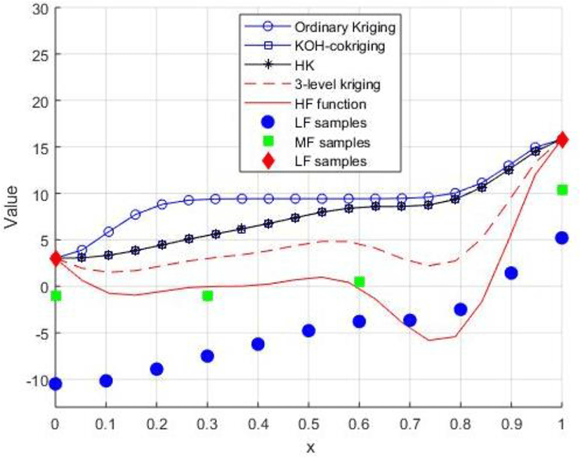
As well as the proposed 3LK is used here to make the comparison among different VFM methods. Fig. 1 shows the results of four different methods for the test case. The solid line represents behavior of the actual model, and the filled diamonds, stars and circles represent given HF, MF and LF sample points, respectively. The dash line represents the result using 3LK model to fit the HF function. It is noted that only 3LK model is built by using sample points of all LF, MF and HF data sets, in contrast, kriging model is built by using 2 HF sample points alone and other models are built by using 11 LF sample points and 2 HF sample points.

Fig. 1. Comparison results of different metamodeling methods.

Download Original Figure

It can be concluded that the proposed 3LK outperforms other methods, since in most locations, it is the closest to the HF function. That is because the MF sample points provide 3LK model more information about HF function to correct the prediction, noting that the number of MF sample points is smaller than LF sample point as well as MF data is cheaper than HF data. The ‘HF data’ is sometimes very expensive or difficult to be extracted in actual engineering data fusion problems. In order to enhance the prediction of HF data when adding more LF sample points does not make more improvement, an additional set of MF data is used to enhance the model. The MAE and MaxAE of different methods are listed in Table 1.

Table 1. Accuracy comparison of various approximation methods (one-dimensional case)

Method	MAE	MaxAE	R ²
Kriging	8.5111	15.2408	0.3076
Co-kriging	6.7748	14.7731	0.3236
HK	6.7842	14.7854	0.3226
3LK	3.7310	8.1480	0.8116

Download Excel Table

2.4. Engineering Case: Construction of Aerodynamic Database for Airfoil Clark Y

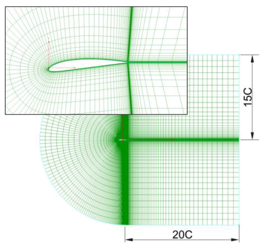
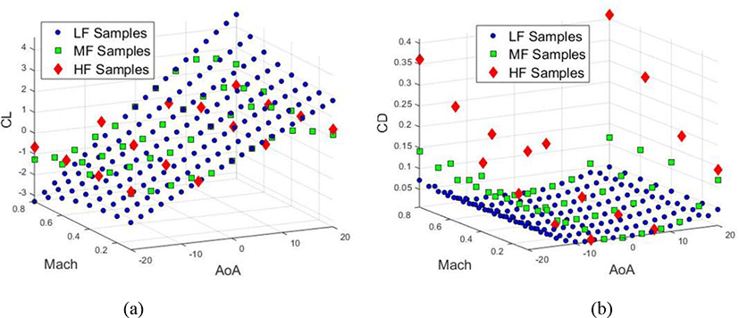
In this section, the validation of proposed method is illustrated through constructing database of the aerodynamic coefficient of an existing airfoil Clark Y. There are two independent variables are considered, such as Mach number,M, and angle of attack, α. The ranges for variables are 0.1 ≤ M ≤ 0.8 and −20° ≤ α ≤ 20°. The database is generated by running independently three different methods, such as Ansys Fluent (16 points), Boundary Layer Method called “BLM” (44 points) and Potential Flow Method called “PFM” (328 points). The data given from Fluent, BLM and PFM are used as the HF, MF and LF sample points, respectively. In this case, the LF and MF sample data are gained by running fast computational algorithms in Javafoil tool, the HF sample data is computed by using Fluent 15.0 simulation tool and Sparlart-Allmaras one-equation turbulent model. The grid consists of about 350,000 elements is used as seen in Fig. 2. It took only minutes for Javafoil runs but approximately 23 h for CFD runs on a 3.0 GHz CPU computer.

Fig. 2. Computation grid for HF model.

Download Original Figure

For training metamodels, the conventional kriging model is constructed by using 16 HF sample points alone. Cokriging, HK, IHK are constructed by using 328 LF sample points and 44 MF sample points. Finally, a 3LK model is constructed by using all mentioned data set. The distributions of various sets of sample data in the design space are shown in Fig. 3 and prediction surfaces of C_L and C_D resulted from various methods are illustrated in Fig. 4. An additional 70 points are randomly selected to verify the accuracy of the built approximate models and results of global and local errors are listed in Table 2.

Fig. 3. Distributions of variable fidelity samples in design space: (a) C_L sample points, (b) C_D sample points.

Download Original Figure

Fig. 4. Surfaces of prediction models from various methods: (a) C_L coefficient (b) C_D coefficient.

Download Original Figure

Table 2. Accuracy comparison of different approximation methods (two-dimensional case)

Method	C_L			C_D
Method	MAE	MaxAE	R ²	MAE	MaxAE	R ²
Kriging	0.4533	1.3197	0.4183	0.0244	0.0871	0.9461
Co-kriging	0.2176	0.8386	0.8609	0.0221	0.0838	0.9032
HK	0.1124	0.6144	0.9530	0.0234	0.0897	0.8918
IHK	0.1560	0.4850	0.9433	0.0216	0.0728	0.9076
3LK	0.1088	0.4297	0.9642	0.0136	0.0502	0.9680

Download Excel Table

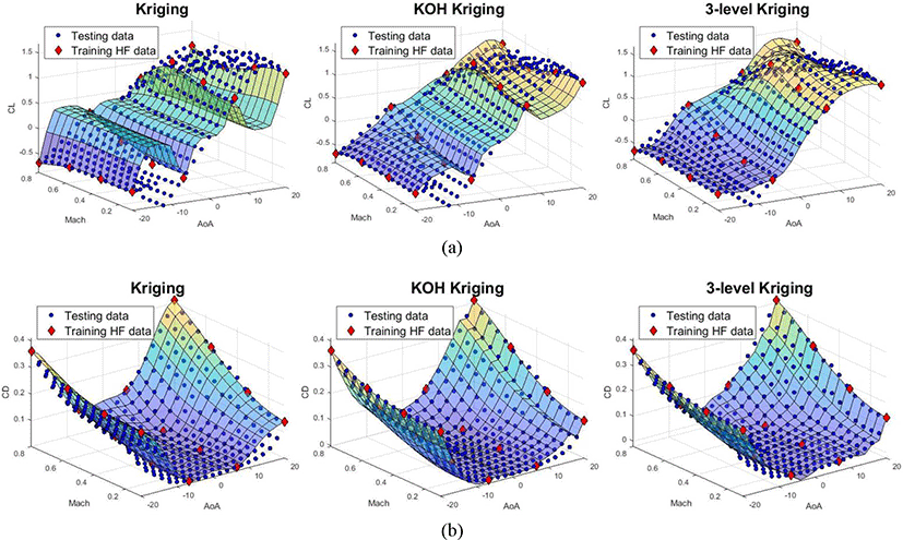
The 3LK model certainly impoves on both the global and local performances compared to ones of other methods. It can also be concluded from Table 2 that the proposed method can provide more accurate metamodel since it has the smallest MAE and Maximum and the largest R² values. It is also proved that developing HK model into 3LK is appropriate choice because HK shows better improvement on both glocal and local performances than ones of other existing methods , though HK is slightly worse than IHK in prediciton of C_D and local performaces in prediciton of C_L. However, global error of HK is much smaller than that of IHK in C_L. It can be undoubted that the key factor making outperformance of 3LK is the additional set of MF sample points, noting that MF sample points are just in a small amount and much cheaper than HF sample points. Indeed, adding only small number of MF sample points, which can more accuratly capture the global trend of HF data, may help significantly improve the performance of metamodel, especially when the number of HF sample points is critically small - a situation in which many of conventional VFM methods may have poor performance. However, this kind of situation is very common in practical problems such as construction of AeroDB in flight simulation application. Another advantage of the proposed method is that it has a more stable performace than other methods when the numer of HF sample points is small. This statement is proved in the next investigation. The Fig. 5 shows the global and local performace of different models in prediciton of C_L with various numbers of HF sample points. In this investigation, an additional number of Fluent sample points are added to train metamodels while reamaining the number of LF and MF sample points.

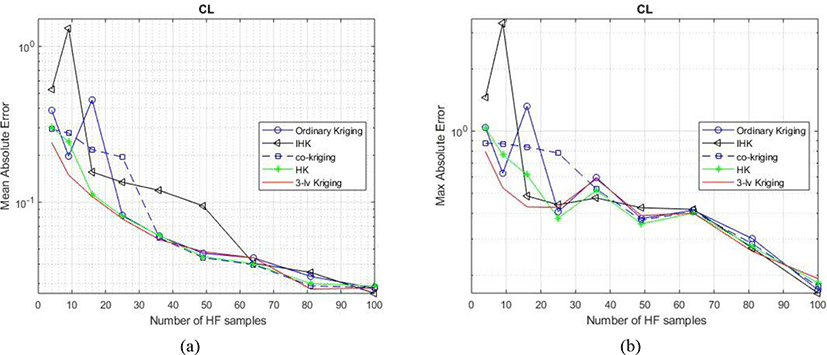
Fig. 5. Accuracy comparison of various methods in C_L prediction with various numbers of HF sample points: (a) MAE, (b) MaxAE.

Download Original Figure

Once again, it can be concluded from figures that the proposed method provides a more accurate and stable metamodel in global and local performances compared to other algorithms, with nearly the smallest MAE, MaxAE and the largest R² with various numbers of HF sample points. The 3LK outperforms from other algorithms in poor condition of small number of HF sample points. In the same condition, ordinary kriging, IHK and co-kriging face poor convergences in both global and local errors. Indeed, only when the number of HF points is more than 36, kriging and co-kriging methods begin to converge into the same fashion as 3LK model does. Although the proposed method may require more computational cost to obtain the MF sample points, this additional computational cost is likely to be offset by the saving in calls required for HF model.

III. CONCLUSION

In this paper, a method for building variable-fidelity metamodel from a hierarchy of data sets with different levels of accuracy is introduced, which is developed from an existing method. This method has more advantages than the origin and allows to improve a surrogate model built on expensive HF data using information from a cheaper one. It is particularly useful when the HF data is very expensive. That is a popular issue in engineering data fusion problems, which mostly require a large amount of data. An example of constructing an aerodynamic database for airfoil Clark Y has been introduced to prove the performance of the proposed method. This work can be extended further to be applied for construction of multidimensional aerodynamic database for actual aircraft in flight simulation applications.

ACKNOWLEDGEMENT

This work was supported by the National Research Foundation of Korea (NRF) [grant NRF-2018R1D1A1B07046779] funded by the Korean government.

REFERENCES

[1].

Forrester, Alexander I. J., Sóbester, and A. J. Keane, Engineering Design via Surrogate Modelling: a Practical Guide, New York, NY: John Wiley & Sons Inc., 2008

[2].

M. C. Kennedy and A. O’Hagan, “Predicting the output from complex computer code when fast approximations are available,” Biometrika, vol. 87, no. 1, pp. 1-13, 2000.

[3].

J. Hu, Q. Zhou, P. Jiang, X. Shao, and T. Xie, “An adaptive sampling method for variable-fidelity surrogate models using improved hierarchical kriging,” Engineering Optimization, vol. 50, no. 1, pp.145-163, 2018.

[4].

Z.-H. Han and S. Gortz, “Hierarchical kriging model for variable-fidelity surrogate modelling,” AIAA Journal, vol. 50, no. 9, September 2012.

[5].

L. Le Gratiet, “Bayesian analysis of hierarchical multi-fidelity codes,” 2012, pp. RSPSA-2011-0742. <hal-00654716v1>

[6].

L. Le Gratiet, “Building kriging models using hierarchical codes with different levels of accuracy,” 11th Annual Meeting of the European Network for Business and Industrial Statistics, Sep 2011, Coimbra, Portugal. <hal-00654710>

[7].

M. Tyan, M. Kim, V. Pham, C. K. Choi, T. L. Nguyen, and J.-W. Lee, “Development of advanced aerodynamic data fusion techniques for flight simulation database construction,” presented at The 2018 Modeling and Simulation Technologies Conference, AIAA AVIATION Forum, (AIAA 2018-3581), Atlanta, Georgia, USA.

[8].

V. Pham, M. Kim, M. Tyan and J.-W. Lee, “A multilevel kriging modeling for variable fidelity aerodynamic database construction,” presented at The KSAS 2018 Fall Conference, Jeju, Korea.

[9].

V. Pham, M. Kim, M. Tyan and J.-W. Lee, “Improved aerodynamic data fusion using local fidelity method for accurate flight simulation,” presented at The KSAS 2019 Spring Conference, Korea.

[10].

L. He, Y. Zhou, W. Qian, and Q. Wang, “Aerodynamic data fusion with a multi-fidelity surrogate modeling method,” 7th European Conference for Aeronautics and Space Sciences (Eucass). doi:

[11].

M. Belyaev, E. Burnaev, E. Kapushev, S. Alestra, M. Dormieux, A. Canvailles, D. Chaillot, and E. Ferreira, “Building data fusion surrogate models for spacecraft aerodynamic problems with incomplete factorial design of experiments,” Advanced Materials Research, vol. 1016, Switzerland: Trans Tech Publications, 2014, pp 405-412.

[12].

T. Chung and K. Gee, and S. Lawrence, “Generation of aerodynamic data using a design of experiment and data fusion approach,” presented at 43rd AIAA Aerospace Sciences Meeting and Exhibit, Reno, Nevada, January 2005

[13].

A. J. Keane, “Wing optimization using design of experiment, response surface, and data fusion methods,” Journal of Aircraft, vol. 40, no. 4, July-August 2003.

[14].

R. T. Haftka, “Combining global and local approximations,” AIAA Journal, vol. 29, no. 9, Septemper 1991.

[15].

N. Cressie, D. M. Hawkins, “Robust estimation of the variogram: I,” Journal of the International Association for Mathematical Geology, 12, 115-125.

[16].

E. R. Unger, M. G. Hutchinson, M. Rais-Rohani, R. T. Haftka, and B. Grossman, “Variable-complexity design of a transport wing,” Intl. J. Systems Automation: Res. and Appl. (SARA), No. 2, 1992, pp. 87-113.

AUTHOR

Vinh Pham

jdaat-1-1-1-i1

Vinh Pham received his BS degree from Dept. of Aerospace Engineering, HCMUT Univ, Ho Chi Minh City, Vietnam in 2016. Currently, he is pursuing his Ph.D. degree in Dept. of Aerospace Information Engineering, Konkuk Univ, Seoul, Korean.

His research interests include numerical optimization and approximation, flight simulation, aircraft design.

Mukyeom Kim

jdaat-1-1-1-i2

Mukyeom Kim received his BS degrees from the Dept of Aerospace Information Engineering, Konkuk Univ, Korea in 2018. He joined the Dept. of Aerospace Information Engineering for his M.S. degree at Konkuk Univ.

His research interests include Optimization, Artificial Intelligence, Gaussian Process Regression, Aerodynamic Analysis and Aerodynamic Data Fusion techniques.

Maxim Tyan

jdaat-1-1-1-i3

Maxim Tyan has obtained his BS degree from Tashkent State Technical University in 2005 and PhD degree from Dept. of Aerospace Information Engineering, Konkuk Univ in 2015.

His research interests include numerical optimization and approximation, flight simulation, aircraft design, and UAV guidance. Currently he is working as a Research Professor in Dept. of Aerospace Information Engineering, Konkuk Univ, Korea.

Jae-Woo Lee

jdaat-1-1-1-i4

Jae-Woo Lee received his Ph.D. from Dept. of Aerospace Engineering, Virginia Tech. U.S. in 1991. He finished M.S. and B.S in Aerospace Engineering, Seoul National University, Seoul, Korea. Currently he is a Professor and Director, Konkuk Aerospace Design-Airworthiness Research Institute, KADA, Konkuk Univ. He is the president of the Korean Society of Design Optimization, KSDO and serves as a vice president of several academic societies including the Korean Society of Aeronautics and Space Science, KSAA, and KOSSE. He is the corresponding author or co-author of over 570 publications including 13 patents and 74 international journal papers. His research interests are Multidisciplinary Design and Optimization, MDO, Aerodynamic Design and Optimization, Aerospace Vehicle Design for Aircraft, Space Launcher, UAV/Drones. He received several honors and awards in his academic career. He has been serving as the conference chair, the technical program chair, and the symposium chair for various international conferences including APISAT, KSAS, KSAA. He served as a Specialized Member at Defense Acquisition Committee, Ministry of National Defense, Korea and at Policy Planning Committee / Business Committee, DAPA, MND, Korea.